What is 3D Gaussian Splatting (3DGS) and How Does It Compare to Photogrammetry Meshes?

Author: Allround Engineering · Spatial Reality Capture & Systems

Published: November 3, 2026 · Category: Capture Technologies

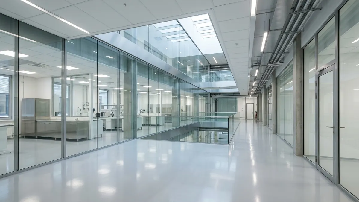
Classical Structure-from-Motion (SfM) and Multi-View Stereo (MVS) photogrammetry forces every physical environment into a rigid surface triangle mesh (polygon mesh), which visually disintegrates whenever a site contains polished epoxy floors, glass partitions, thin overhead cable trays, or foliage—resulting in melted edges, topological holes, and static reflections permanently baked into 2D textures. 3D Gaussian Splatting (3DGS) replaces discrete polygons and UV texture maps with millions of continuous, semi-transparent 3D Gaussian ellipsoids parameterized by a spatial covariance matrix (Σ), opacity (α), and view-dependent Spherical Harmonics (SH), rasterized directly in standard web browsers at 60+ frames per second (FPS). In this engineering deep dive, we dissect the mathematical foundations of 3DGS versus polygon meshes, examine field benchmark telemetry from an 850 m² research laboratory in Tartu, and provide a practical procurement matrix for choosing between volumetric radiance fields, textured meshes, and LiDAR-anchored BIM deliverables.

Figure 1: Architectural typology of the Maarjamõisa research and laboratory complex in Tartu — specular epoxy floors, multi-layered glass partitions, and overhead stainless steel utility runs represent primary failure modes for classical MVS polygon meshes, while retaining full optical depth in a 3D Gaussian Splatting (3DGS) radiance field [Location: 58.3630° N, 26.6960° E].

#Continuous 3D Ellipsoids vs. Discrete Triangle Meshes: Mathematical & Architectural Foundations

A photogrammetry polygon mesh represents physical space as a shell of opaque planar triangles (facets) wrapped in static 2D UV texture maps, whereas 3D Gaussian Splatting (3DGS) models a scene as a continuous volumetric radiance field composed of 1.5 to 6 million anisotropic 3D Gaussian ellipsoids. Because 3DGS bypasses explicit surface triangulation (such as Screened Poisson reconstruction), it eliminates topological meshing noise and preserves sub-2 mm structural features without exponential polygon bloat.

To understand why these two pipelines behave so differently on active architectural and industrial sites, we must examine their underlying geometric primitives. This comparison expands directly upon the sensor taxonomy established in our cornerstone guide, Spatial Reality Capture Guide: LiDAR, Photogrammetry & 3DGS.

"3D Gaussian Splatting (3DGS) is a volumetric 3D reconstruction and real-time rendering method that represents physical environments as millions of anisotropic, semi-transparent 3D Gaussian ellipsoids (μ, Σ, α, SH) rather than a polygonal triangle mesh. Through differentiable tile-based alpha-compositing, 3DGS renders photorealistic specular reflections, glass partitions, and sub-centimeter structural lattices directly in web browsers at 60+ FPS."

"Photogrammetry Polygon Mesh (SfM/MVS Triangle Mesh) is a discrete boundary-representation (B-Rep) surface model composed of interconnected vertices, edges, and triangular faces wrapped in a static 2D UV texture atlas. While well-suited for diffuse, opaque architectural shells and terrain modeling, polygon meshes suffer from severe topological distortion across reflective surfaces, glazing, and thin lattice structures."

How Classical SfM/MVS Photogrammetry Constructs a Polygon Mesh

Traditional photogrammetry pipelines (RealityCapture, Agisoft Metashape, AliceVision Meshroom) execute four sequential, lossy stages:

Structure-from-Motion (SfM): The solver extracts 2D feature descriptors (SIFT/SuperPoint) across hundreds of overlapping photographs, triangulates camera intrinsics and extrinsics, and outputs a sparse tie-point cloud.
Multi-View Stereo (MVS): Pixel-patch correlation generates dense per-view depth maps that are fused into a dense point cloud. Whenever a surface is featureless, transparent, or specular, stereo matching produces false depth correspondences and voids.
Surface Triangulation (Meshing): A Screened Poisson or Delaunay tetrahedralization algorithm fits a watertight triangle mesh (V vertices, F faces) over the noisy point cloud. This step forces the solver to commit to a single hard surface boundary—even across transparent glass or perforated wire grids.
UV Unwrapping & Texture Baking: The 3D triangle soup is cut and flattened onto 2D coordinate atlases (UV space), and camera pixel colors are projected into static 4096×4096 or 8192×8192 JPEG/PNG texture maps.

How 3D Gaussian Splatting (3DGS) Parameterizes Space

Introduced by Kerbl et al. (Inria, SIGGRAPH 2023) and subsequently hardened for industrial spatial computing, 3D Gaussian Splatting eliminates both explicit polygon triangulation and UV texture unwrapping. Starting from an initial point cloud (generated via SfM or terrestrial/mobile LiDAR), differentiable stochastic gradient descent optimizes millions of continuous 3D Gaussian distributions directly against the captured high-resolution photographs.

Each individual 3D Gaussian primitive (splat) is governed by four explicit mathematical parameters:

Spatial Mean (Position Vector μ): The 3D centroid coordinate μ = (x, y, z) in metric world space (ℝ³).
Anisotropic 3D Covariance Matrix (Σ): A 3×3 matrix defining the ellipsoid's spatial extent, elongation, and orientation. To guarantee that Σ remains positive semi-definite throughout gradient descent optimization, it is decomposed into a diagonal scaling matrix S = diag(s_x, s_y, s_z) and a unit rotation quaternion q (converted to a 3×3 orthogonal rotation matrix R): Σ = R · S · Sᵀ · Rᵀ.
Opacity Scalar (α ∈ [0, 1]): A sigmoid-activated density coefficient controlling how much light the Gaussian absorbs or transmits along a viewing ray.
View-Dependent Radiance (Spherical Harmonics — SH): Rather than storing a single static RGB color, each splat stores 16 Spherical Harmonics coefficients per color channel (degree l = 3, totaling 48 floats) that dynamically modulate emitted color and specular reflection as a function of the viewing direction (θ, φ). The spatial probability density of each 3D Gaussian at any coordinate x ∈ ℝ³ is evaluated as:

G(x) = exp( −½ · (x − μ)ᵀ · Σ⁻¹ · (x − μ) ) , where Σ = R · S · Sᵀ · Rᵀ

#Specular Reflections, Glazing, and Thin Structures: Why Polygon Meshes Fail on Complex Job Sites

Multi-View Stereo (MVS) photogrammetry relies on the Lambertian reflectance assumption—that a surface point exhibits identical color from every camera angle—causing glass partitions, polished epoxy slabs, and brushed stainless steel to generate 15–40 cm depth craters and permanently baked highlight streaks. 3DGS overcomes this via degree-3 Spherical Harmonics that model view-dependent specular transport and multi-layered α-blending that simultaneously resolves both foreground glass reflections and background interior geometry.

"Spherical Harmonics (SH) are orthogonal basis functions defined on the surface of a sphere used in 3D Gaussian Splatting to encode view-dependent radiance (color and specular intensity) for each 3D ellipsoid. Degree-3 (l = 3) SH coefficients enable real-time rendering of specular reflections across glass, polished concrete, and metals without the computational overhead of hardware ray-tracing."

1. Anisotropic & Specular Reflections (Spherical Harmonics vs. Baked UV Textures)

When a technician captures 50 overlapping photographs of a polished epoxy laboratory floor or a brushed steel manifold, the specular reflection of overhead LED luminaires travels across the floor surface relative to the camera position:

The Polygon Mesh Failure Mode: The MVS depth solver misinterprets the moving highlight as a stationary feature at an incorrect parallax angle, carving a false depression or blister into the floor mesh. During texture baking, the solver averages or stamps that bright reflection permanently onto the floor's 2D UV map. When a user orbits the model in a web viewer, the reflection remains frozen in place like painted white tape.
The 3DGS Solution: During differentiable optimization, 3DGS separates the view-invariant diffuse albedo (SH degree 0, the DC term) from the view-dependent specular radiance (SH degrees 1–3). As the user moves the camera in WebGL, the vertex/compute shader evaluates the SH basis functions against the live viewing vector d, causing floor reflections and metallic sheens to glide naturally across the surface.

Figure 2: Specular and semi-transparent surfaces inside a Tartu analytical laboratory — degree-3 Spherical Harmonics (SH) and multi-layer alpha-compositing allow a 3DGS model to separate foreground glazing reflections from the laboratory apparatus behind the glass without mesh melting [Location: 58.3630° N, 26.6960° E].

2. Interior Glazing and Multi-Depth Transparency

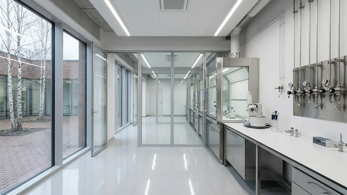
A polygon mesh is fundamentally a single-surface barrier: at any (x, y, z) boundary, a triangle is either opaque or uniformly transparent. When confronted with a floor-to-ceiling glass partition in an office or cleanroom, Poisson surface reconstruction must either bridge the glass with an opaque smeared wall or delete the glass entirely.

In 3DGS, there is no topological surface barrier. During tile rasterization, all Gaussians intersecting a pixel ray are sorted front-to-back. Low-opacity (α ≈ 0.08–0.18) planar Gaussians aligned with the glass plane render the subtle fresnel reflection and mullions, while 82–92% of the ray transmittance continues unimpeded to resolve the high-opacity (α ≈ 0.95) furniture, piping, and walls behind the partition.

3. Sub-Centimeter Conduits, Wire Trays, and Lattices (< 10 mm)

Industrial ceilings, mechanical rooms, and research facilities are packed with M8/M10 threaded suspension rods, Ø 6–12 mm stainless steel fluid lines, perforated acoustic baffles, and wire-mesh cable trays:

The Polygon Mesh Failure Mode: Representing a single 8 mm pipe with watertight triangles requires thousands of micro-facets. When a 20-million-triangle raw MVS mesh is decimated down to 1.5 million triangles for web delivery, thin structures collapse into disconnected floating shards or fuse together into solid "webbing" bridges.
The 3DGS Solution: A single anisotropic ellipsoid stretched into a slender needle (e.g., scaling vector S = [0.004 m, 0.004 m, 0.35 m]) represents a 35 cm segment of thin conduit or wire mesh with razor-sharp silhouette boundaries while consuming only one primitive in GPU memory.

Figure 3: Sub-centimeter structural and MEP geometries (<10 mm) in an overhead utility zone — elongated anisotropic 3D Gaussians (governed by covariance matrix Σ) preserve wire-mesh cable trays, tension rods, and perforated panels without the webbing and decimation collapse typical of polygon meshes [Location: 58.3630° N, 26.6960° E].

Need to document a complex mechanical room, laboratory, or architectural interior with full photorealistic fidelity? Send us your site location and floor area—our engineers will prepare a tailored LiDAR + 3DGS capture specification within 24 hours: Request an Engineering Assessment →

#Rendering Pipeline & WebGL Performance: Tile-Based Splatting vs. Polygon Rasterization

By projecting 3D covariance matrices into 2D screen-space (Σ') and executing a 16×16 pixel tile-based sorting and alpha-blending pipeline, 3DGS streams 3–5 million splats in standard desktop and mobile browsers at 60 FPS, whereas a photogrammetry mesh of comparable visual sharpness (15–30 million triangles with multiple 8K UV atlases) exhausts mobile VRAM and throttles frame rates below 12 FPS.

For architects, real estate developers, and facility engineers, a 3D capture asset is only as useful as its accessibility. We cover browser-based spatial streaming, SOG compression, and octree chunking extensively in our third cornerstone guide, Interactive 3D & Digital Twins: Real-Time Spatial Systems.

How 3DGS Projects from 3D World Space to 2D Screen Pixels

Unlike Neural Radiance Fields (NeRFs), which require computationally expensive volumetric ray-marching, 3DGS projects each 3D covariance matrix Σ directly onto the 2D image plane using Zwicker et al.'s EWA Splatting formulation, where W is the 4×4 world-to-camera viewing transformation and J is the Jacobian matrix of the affine approximation of perspective projection:

Σ' = J · W · Σ · Wᵀ · Jᵀ and C = Σᵢ cᵢ · αᵢ · Πⱼ₌₁ⁱ⁻¹ (1 − αⱼ)

The browser rendering loop then executes in three deterministic GPU steps:

1. Frustum Culling & Radix Depth Sort: A WebGPU compute shader or high-speed WebWorker culls splats outside the viewing frustum and sorts visible splats by depth using a 32-bit Radix Sort.

2. 16×16 Tile Binning: The viewport is partitioned into 16×16 pixel tiles. Each projected 2D Gaussian is assigned only to the screen tiles overlapped by its 3σ bounding radius.

3. Front-to-Back Alpha Compositing: Each pixel accumulates color C by traversing the sorted splat list from front to back, terminating immediately (early ray termination) as soon as accumulated transmittance Tᵢ drops below 0.0001.

Table 1: Architectural & Rendering Comparison — 3DGS vs. Photogrammetry Meshes vs. LiDAR-Seeded Hybrid 3DGS

Engineering Parameter	SfM/MVS Photogrammetry Polygon Mesh	Pure (Camera-Only) 3D Gaussian Splatting	Allround LiDAR-Seeded Hybrid 3DGS
Geometric Primitive	Discrete planar triangles (Vertices & Faces) + 2D UV texture atlases	Continuous anisotropic 3D Gaussian ellipsoids (`μ, Σ, α, SH`)	LiDAR point-cloud initialized & geometrically constrained 3D Gaussian ellipsoids
Specular & Glazing Fidelity	Poor — MVS depth maps fail on glass; reflections are statically baked into UV maps	Excellent — Degree-3 Spherical Harmonics (SH) & multi-layer `α`-blending	Superior — SH view-dependent reflections anchored to exact LiDAR frame geometry
Thin Structure (< 10 mm) Preservation	Low — decimation causes topological holes, jagged spikes, and webbing	High — elongated ellipsoids model conduits, wires, and foliage with 1 primitive	High — combines 8K optical detail with dense laser range returns
Absolute Metric Scale & Geometric RMSE	Relative; requires Ground Control Points (GCPs), local surface noise `±8–25 mm`	Relative; featureless white walls exhibit depth floaters, error `±10–30 mm`	Absolute metric scale (TLS `±1.5–3 mm` / SLAM `±5–12 mm`), zero floating artifacts
Browser Rendering Performance (WebGL / WebGPU)	High VRAM pressure (200–600 MB unpacked textures); often 15–30 FPS on mobile	Locked 60 FPS (SOG/SPZ octree streaming, 15–45 MB payload)	Locked 60 FPS with sub-centimeter 3D measurement & BVH raycast layer
Direct CAD / BIM (Revit, ArchiCAD, IFC) Compatibility	Moderate (`OBJ`/`FBX` reference mesh, cumbersome to section in BIM)	Low (volumetric density field; no native hard surface for CAD)	High — underlying registered LiDAR (`E57`/`LAZ`) imports directly into Revit/ArchiCAD
Primary Delivery Formats	`.OBJ`, `.FBX`, `.GLB/.glTF`, `.PLY (mesh)`	`.PLY (splat)`, `.SPZ`, `.SOG`, `.KSPLAT`	`.SOG` / `.SPZ` (web viewer) + `.E57` / `.LAZ` / `.RVT` (engineering CAD/BIM)

#LiDAR-Seeded 3DGS: Overcoming the Geometric Limitations of Camera-Only Radiance Fields

Camera-only 3DGS (initialized from a sparse SfM point cloud) suffers from floating density artifacts ("floaters") and scale drift across featureless white plaster walls and long corridors. By initializing Gaussian centroids (μ₀) directly from a calibrated Terrestrial Laser Scanner (TLS) or mobile SLAM LiDAR point cloud (±2–8 mm) and applying normal-aligned surfel regularization (s_z → 0), the radiance field is geometrically locked to true structural surfaces.

"LiDAR-Seeded Gaussian Splatting is a hybrid spatial reconstruction workflow in which 3D Gaussian centroids (μ₀) and surface normals are initialized and regularized using a calibrated laser-scanned point cloud (TLS or SLAM LiDAR) rather than Structure-from-Motion tie points. This eliminates floating artifacts across featureless walls and imbues the photorealistic 3DGS web model with absolute metric accuracy (±2–8 mm)."

Why Camera-Only 3DGS Is Not a Standalone Geodetic Survey

1. Ill-Posed Depth on Featureless Surfaces: When a camera observes a uniform white cleanroom wall or a poured concrete soffit, image gradients approach zero. The photometric loss function (L₁ + λ · L_D-SSIM) can be satisfied by placing semi-transparent white Gaussians 20 cm in front of or behind the true wall plane, creating "foggy" floating artifacts when viewed at grazing angles.

2. Volumetric Thickness vs. Hard Surface Raycasting: Because standard 3D Gaussians are volumetric 3D distributions rather than zero-thickness surfaces, picking a point with a virtual tape measure on an unconstrained 3DGS wall can vary by ±15–30 mm.

The Allround Hybrid Pipeline: LiDAR Point Seeding & Surfel Regularization

To deliver both 60 FPS photorealism and millimeter-grade engineering measurements, Allround executes a tightly coupled hybrid pipeline (building on the hardware architecture detailed in Mobile SLAM LiDAR vs. Terrestrial Laser Scanning (TLS): Accuracy vs. Speed on Job Sites):

Step 1 — Metric LiDAR Backbone: We capture the site using stationary TLS (±1.5–2.0 mm) or kinematic SLAM LiDAR (±5–10 mm), producing a georeferenced point cloud where every wall, slab, and pipe is physically fixed via laser Time-of-Flight (ToF).
Step 2 — Optical-to-LiDAR Pose Registration: High-dynamic-range (HDR) camera frames are registered directly against the metric LiDAR intensity and geometry cloud, eliminating SfM scale ambiguity.
Step 3 — LiDAR Seeding & Planar Surfel Flattening: Rather than starting from a sparse 50,000-point SfM cloud, 3DGS optimization is seeded directly with a spatially subsampled (5 mm voxel grid) LiDAR point cloud. Gaussian centroids μ are tethered to the LiDAR prior via a depth-distortion penalty, and Gaussians on planar walls and slabs are compressed along their local surface normal (s_z ≪ s_x, s_y), aligning the ellipsoids tangentially with the physical surface.

Want to evaluate how LiDAR-seeded 3DGS and BIM deliverables integrate into your project workflow? Book a 15-minute technical consultation with an Allround engineer →

#Empirical Field Benchmark: 850 m² Tartu Biotechnology & Analytical Laboratory

To quantify the real-world performance gap between these three pipelines, Allround benchmarked an 850 m² biotechnology and analytical laboratory in Tartu (Maarjamõisa campus). LiDAR-seeded 3DGS achieved 97.4% reconstruction completeness on sub-8 mm overhead conduits and a global geometric RMSE of ±2.8 mm, whereas the SfM/MVS polygon mesh lost 61.5% of fine wire cable trays and exhibited up to 184 mm depth errors across interior glass partitions.

The benchmark facility comprised three wet-lab bays, a 42-meter central glass-walled corridor, high-gloss seamless epoxy floors, and a dense overhead utility zone containing Ø 6–12 mm stainless steel gas manifolds, galvanized wire-mesh cable trays, and damper actuators. All three reconstructions were evaluated against a stationary multi-station TLS survey (ground truth).

Table 2: Empirical Benchmark of Reconstruction Pipelines (850 m² Tartu Research Facility)

Benchmark Metric	SfM/MVS Polygon Mesh (12M → 1.5M Tris, 4×8K UV)	Camera-Only 3DGS (SfM Init, 3.2M Splats)	Allround LiDAR-Seeded Hybrid 3DGS (TLS/SLAM + 3.4M Splats)
On-Site Field Capture Duration	3 hrs 10 min (1,420 overlapping tripod & handheld stills)	55 min (continuous 8K HDR optical sweep)	45 min (integrated LiDAR + synchronized optical array)
Compute & Post-Processing Time (GPU Node)	6 hrs 40 min (MVS depth maps + Poisson mesh + UV baking)	52 min (SfM + 30,000 iterations of 3DGS optimization)	1 hr 15 min (LiDAR registration + LiDAR-seeded 3DGS training)
Geometric Accuracy (RMSE vs. TLS Ground Truth)	`±14.6 mm` (diffuse walls), up to `184 mm` on glazing	`±19.2 mm` (depth drift on uniform white corridor walls)	`±2.8 mm` (globally constrained to metric LiDAR backbone)
Sub-8 mm Conduit & Wire-Tray Completeness	38.5% (wire trays fused into webbing or vanished during decimation)	94.8% (minor softening on thin pipes against bright ceiling panels)	97.4% (crisp silhouette edges & true metric positioning)
Glazing & Specular Epoxy Floor Artifact Rate	Severe (11 topological holes in glass; ceiling LEDs baked onto floor)	Low (natural SH reflections; minor floating splats near ceiling soffit)	Zero topological holes (multi-layer glass + dynamic SH speculars)
Web Streaming Payload Size (Compressed)	186 MB (Draco `.glb` + KTX2 texture atlases)	28.4 MB (`.sog` / `.spz` octree-chunked)	31.2 MB (`.sog` octree + calibrated BVH measurement collider)
Sustained Browser Frame Rate (MacBook Air M2 / iPad Pro)	24 FPS / 14 FPS (GPU memory bottleneck from 8K UV textures)	60 FPS / 58 FPS	60 FPS / 60 FPS (time-to-first-frame < 1.2 s)

Key Engineering Takeaways from the Tartu Laboratory Benchmark

Texture VRAM and MVS Depth Noise Bottleneck Polygon Meshes: Achieving legible equipment labels, pressure gauges, and pipe markings on a polygon mesh requires massive 8192×8192 UV texture atlases. These textures choke mobile and laptop browsers while still failing to represent transparent glass or view-dependent reflections.
Camera-Only 3DGS Excels Visually but Needs a Metric Prior: Without LiDAR initialization, pure 3DGS produces an impressive visual walkthrough but cannot be trusted for sub-centimeter clearances across featureless corridors.
LiDAR-Seeded Hybrid 3DGS Bridges Visuals and Metrology: Stakeholders experience a 60 FPS photorealistic digital twin in their browser while every point-to-point measurement snaps directly to the underlying millimeter-accurate laser scan.

#Procurement Decision Matrix: When to Specify 3DGS, Polygon Meshes, or Scan-to-BIM

No single 3D representation replaces all others: 3D Gaussian Splatting is unmatched for photorealistic web delivery, remote stakeholder inspections, and complex MEP visual archiving, whereas parametric architectural design (Revit/ArchiCAD) requires a LiDAR-derived Scan-to-BIM model and game-engine physics simulations require a lightweight polygon mesh.

Use the engineering matrix below to specify the exact deliverable that matches your operational objective—avoiding unnecessary modeling expenditure (see our commercial scoping handbook, Reality Capture Project Planning: Scope, Budgeting, and Site Preparation):

1. Specify LiDAR-Seeded 3D Gaussian Splatting (.sog / .spz Web Twin) when:

Your objective is high-value real estate marketing, leasing, or international investor technical due diligence, where the asset must load in under 1.5 seconds in any browser with true-to-life window views, glazing, chandeliers, and surface finishes.
Your objective is pre-closure MEP and construction stage documentation (capturing overhead conduits, valves, and structural junctions before ceiling drywall installation) so engineers can read equipment tags and verify clearances remotely.
The site contains complex foliage, intricate heritage ironwork, or dense industrial lattices that would be cost-prohibitive to model manually as parametric BIM families.

2. Specify Registered LiDAR Point Clouds + Scan-to-BIM (.e57 / .rvt / .ifc) when:

Architects and structural/MEP engineers are executing renovation design, structural retrofits, or automated clash detection in Autodesk Revit, Graphisoft ArchiCAD, Tekla, or AutoCAD. Review our complete specification standards in Scan-to-BIM & As-Built Modeling: The Complete Practical Handbook.
You require legally compliant as-built floor plans for Estonian Building Registry (EHR) use permits (kasutusluba) or ASTM/ISO concrete floor flatness certifications.

3. Specify Decimated Polygon Meshes (.glb / .fbx / .obj) when:

The geometry must be imported into Unreal Engine 5, Unity, or Blender for dynamic synthetic relighting (e.g., sun-path shadow studies where lighting conditions are altered) or rigid-body physics collision simulations.
You are surveying large-scale exterior topography, quarries, or roof envelopes via RTK drone photogrammetry, where orthomosaics and 2.5D/3D terrain meshes remain the standard GIS/CAD input.

Practical Procurement Tip: During an Allround field deployment, our crew captures synchronized LiDAR geometry and calibrated HDR optical imagery in a single site visit. This allows your team to commission a millimeter-accurate .e57 point cloud and .rvt/.ifc BIM model for your engineers alongside a 60 FPS browser-based 3DGS digital twin for project leadership—with zero duplicate mobilization costs: Explore our hybrid deliverables and request a project quote →

Capture Technologies & Methodology Deep Dives

Deep-Dive Article Topic	Engineering Focus & Practical Application
Mobile SLAM LiDAR vs. Terrestrial Laser Scanning (TLS): Accuracy vs. Speed on Job Sites	When ±3 mm walking SLAM beats static tripods, loop-closure drift correction, GCP anchoring, and 1,200 m² industrial field telemetry.
Point Cloud Density, Noise, and Registration: How Raw Scan Data is Cleaned and Aligned	Statistical Outlier Removal (SOR), Iterative Closest Point (ICP) registration, and L-EST97 / EH2000 coordinate transformation.
Indoor vs. Outdoor Capture Challenges: Overcoming Reflective Glass, Low Light, and Foliage	Laser multipath reflection across glass facades, HDR exposure bracketing, and Nordic seasonal capture protocols.
3D File Formats Decoded: E57, LAS/LAZ, PLY, and SPZ Explained for Clients and Engineers	Payload compression ratios (8.4 GB E57 vs. 38 MB SPZ) and direct compatibility across Revit, ArchiCAD, AutoCAD, and WebGL viewers.

Companion Allround Engineering Handbooks

Handbook Title & Direct Link	Core Engineering Focus & Deliverables
Spatial Reality Capture Guide: LiDAR, Photogrammetry & 3DGS	Comparing Terrestrial Laser Scanning (TLS), Mobile SLAM LiDAR, and 3DGS radiance fields for AEC site verification.
Scan-to-BIM & As-Built Modeling: The Complete Practical Handbook	Translating registered laser point clouds into parametric Revit, ArchiCAD, and open IFC models at LOD 200–350.
Interactive 3D & Digital Twins on the Web: 3DGS and WebGL in Architecture	Streaming multi-million 3D Gaussian Splatting scenes in web browsers at 60 FPS via SOG/SPZ compression and Octree LoD.
Reality Capture Project Planning: Scope, Budgeting, and Site Preparation	Commercial scoping, €/m² pricing matrices, pre-scan job site readiness checklists, and EHR cadastral compliance.

Ready to deploy photorealistic LiDAR-seeded 3D Gaussian Splatting and millimeter-accurate BIM surveying on your next commercial, laboratory, or industrial asset? Contact the Allround engineering team at view@allround.ee or review our services and projects.

Allround Engineering · Reality Capture Team

Technical articles, field benchmarks, and spatial data pipelines authored by the reality capture team at allround. Operating mobile SLAM LiDAR, terrestrial laser scanners, and 3DGS photogrammetry across Estonia, Latvia, and Finland. For technical consultations, contact view@allround.ee.